

You most likely use Google every day, and these days, you might need observed AI-powered search outcomes that compile solutions from a number of sources. However you might need questioned how the AI can collect all this data and reply at such blazing speeds, particularly when in comparison with the medium-sized and huge fashions we usually use. Smaller fashions are, in fact, sooner in response, however they aren’t educated on as massive a corpus as greater parameter fashions.
Therefore, a number of approaches have been proposed to hurry up responses, corresponding to Combination of Consultants, which prompts solely a subset of the mannequin’s weights, making inference sooner. On this weblog, nonetheless, we are going to deal with a very efficient technique that considerably hurries up LLM inference with out compromising output high quality. This method is called Speculative Decoding.
What usually occurs?
In a typical LLM technology course of, we undergo two major steps:
- Ahead Move
- Decoding Part
The 2 steps work as follows:
- Through the ahead move, the enter textual content is tokenised and fed into the LLM. Because it passes by means of every layer of the mannequin, the enter will get remodeled, and ultimately, the mannequin outputs a likelihood distribution over attainable subsequent tokens (i.e., every token with its corresponding likelihood).
- Through the decoding part, we choose the following token from this distribution. This may be achieved both by selecting the best likelihood token (grasping decoding) or by sampling from the highest possible tokens (top-p or nucleus sampling kinda).
As soon as a token is chosen, we append it to the enter sequence(prefix string) and run one other ahead move by means of the mannequin to generate the following token. So, if we’re utilizing a big mannequin with, say, 70 billion parameters, we have to carry out a full ahead move by means of your entire mannequin for each single token generated. This repeated computation makes the method time-consuming.
In easy phrases, autoregressive fashions work like dominoes; token 100 can’t be generated till all of the previous tokens are generated. Every token requires a full ahead move by means of the community. So, producing 100 tokens at 20 ms per token leads to a couple of 2-second delay, and every token should watch for all earlier tokens to be processed. That’s fairly costly when it comes to latency.
How Speculative Decoding helps?
Right here, we use two fashions: a big LLM (the goal mannequin) and a smaller mannequin (usually a distilled model), which we name the draft mannequin. The important thing concept is that the smaller mannequin shortly proposes tokens which can be simpler and extra predictable (like widespread phrases), whereas the bigger mannequin ensures correctness, particularly for extra complicated or nuanced tokens (corresponding to domain-specific phrases).
In different phrases, the smaller mannequin approximates the behaviour of the bigger mannequin for many tokens, however the bigger mannequin acts as a verifier to keep up total output high quality.
The core concept of speculative decoding is:
- Draft – Generate Okay tokens shortly utilizing the smaller mannequin
- Confirm – Run a single ahead move of the bigger mannequin on all Okay tokens in parallel
- Settle for/Reject – Settle for right tokens and substitute incorrect ones utilizing rejection sampling
Word: This technique was proposed by Google Analysis and Google DeepMind within the paper “Accelerating LLM Decoding with Speculative Decoding.”
Diving Deeper
We all know {that a} mannequin usually generates one token per ahead move. Nonetheless, we are able to additionally feed a number of tokens into an LLM and have them evaluated in parallel, unexpectedly, inside a single ahead move. Importantly, verifying a sequence of tokens is roughly comparable in price to producing a single token whereas producing a likelihood distribution for every token within the sequence.
Mp = draft mannequin (smaller mannequin)
Mq = goal mannequin (bigger mannequin)
pf = prefix (the present string to finish the sequence)
Okay = 5 (variety of tokens to draft in a single ahead move)
1) Draft Part
We first run the draft mannequin autoregressively for Okay (say 5) steps:
p1(x) = Mp(pf) → x1
p2(x) = Mp(pf, x1) → x2
…
p5(x) = Mp(pf, x1, x2, x3, x4) → x5
At every step, the mannequin takes the prefix together with beforehand generated tokens and outputs a likelihood distribution over the vocabulary (corpus). We then pattern from this distribution to acquire the following token, identical to in the usual decoding course of.
Let’s assume our prefix string to be:
pf = “I like SRH since …”
Right here, p(x) represents the draft mannequin’s confidence for every token from its current vocabulary.
| Token | x₁ | x₂ | x₃ | x₄ | x₅ |
| they | have | Bhuvi | and | Virat | |
| p(x) | 0.9 | 0.8 | 0.7 | 0.9 | 0.7 |
That is the assumed likelihood distribution we bought from our draft mannequin. Now we transfer to the following step…
2) Confirm Part
Now that now we have run the draft mannequin for Okay steps to get a sequence of Okay(5) tokens. Now we should run our goal mannequin (massive mannequin) as soon as in parallel. The goal mannequin might be fed the pf string and all of the tokens generated by the draft mannequin, since it should examine all these tokens in parallel, and it’ll generate for us one other set of 5 likelihood distributions for every of the 5 generated tokens.
q1(x), q2(x), q3(x), q4(x), q5(x), q6(x) = Mq(pf, x1, x2, x3, x4, x5)
Right here, qi(x) stands because the goal mannequin’s confidence that the drafted tokens are right.
| Token | x₁ | x₂ | x₃ | x₄ | x₅ |
| they | have | Bhuvi | and | Virat | |
| p(x) | 0.9 | 0.8 | 0.7 | 0.8 | 0.7 |
| q(x) | 0.9 | 0.8 | 0.8 | 0.8 | 0.2 |
You may discover q6(x); we’ll come again to this shortly. 🙂
Keep in mind: – We’re solely producing distributions for the goal mannequin; we’re not sampling from these distributions. All the tokens we pattern from are from the draft mannequin, not the goal mannequin initially.
3) Settle for / Reject (Instinct)
Subsequent is the rejection sampling step, the place we resolve which tokens we attempt to preserve and which to reject. We are going to loop by means of every token one after the other, evaluating the p(x) and q(x) chances that the respective draft and goal mannequin have assigned.
We might be accepting or rejecting primarily based on a easy if-else rule. For now, let’s simply get a easy understanding of how rejection sampling occurs, then let’s dive deeper. Realistically, this isn’t how this works out, however let’s go forward for now… We will cowl this factor within the following part.
Case 1: if q(x) >= p(x) then settle for the token
Case 2: else reject
| Token | x₁ | x₂ | x₃ | x₄ | x₅ |
| they | have | Bhuvi | and | Virat | |
| p(x) | 0.9 | 0.8 | 0.7 | 0.8 | 0.7 |
| q(x) | 0.9 | 0.8 | 0.8 | 0.8 | 0.2 |
| ✅ | ✅ | ✅ | ✅ | ❌ |
So right here we see 0.9 == 0.9, so we settle for the “they” token and so forth till the 4th-draft token. However as soon as we attain the fifth draft token, we see now we have to reject the “Virat” token for the reason that goal mannequin isn’t very assured in what the draft mannequin has generated right here. We settle for tokens till we encounter the primary rejection. Right here, “Virat” is rejected for the reason that goal mannequin assigns it a a lot decrease likelihood. The goal mannequin will then substitute this token with a corrected one.
So, the situation that now we have visualised is the virtually best-case situation. Let’s see the worst-case and finest case situation utilizing the tabular type.
Worst Case Situation
| Token | x₁ | x₂ | x₃ | x₄ | x₅ |
| okay | group | they | have | there | |
| p(x) | 0.8 | 0.9 | 0.6 | 0.7 | 0.8 |
| q(x) | 0.3 | 0.6 | 0.5 | 0.7 | 0.9 |
| ❌ | ❌ | ❌ | ❌ | ❌ |
Right here, on this situation, we witness that the primary token is rejected itself, therefore we should break free from the loop and discard all the next tokens too (now not related, therefore discarded). Since every token is expounded to its previous token. After which the goal mannequin has to right the x1 token, after which once more the draft mannequin will draft a brand new set of 5 tokens and the goal mannequin verifies it, and so the method proceeds.
So, right here within the worst-case situation, we are going to generate just one token at a time, which is equal to us operating our activity with the bigger mannequin, usually just like normal decoding, with out adopting speculative decoding.
Finest Case Situation
| Token | x₁ | x₂ | x₃ | x₄ | x₅ |
| they | have | Bhuvi | and | David | |
| p(x) | 0.9 | 0.8 | 0.7 | 0.8 | 0.7 |
| q(x) | 0.9 | 0.8 | 0.8 | 0.8 | 0.9 |
| ✅ | ✅ | ✅ | ✅ | ✅ |
Right here, in one of the best case situation, we see all of the draft tokens have been accepted by the goal mannequin with flying colours and on prime of this. Do you keep in mind after we questioned why the q6(x) token was generated by the goal mannequin? So right here we are going to get to learn about this.
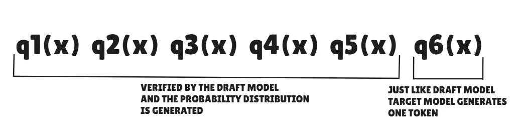
So mainly, the goal mannequin takes within the prefix string, and the draft mannequin generated tokens and verifies them. Together with the goal mannequin’s likelihood distribution, it offers out one token following the x5 token. So, following the tabular instance now we have above, we are going to get “Warner” because the token from the goal mannequin.
Therefore, within the best-case situation, we get Okay+1 tokens at one time. Whoa, that’s an enormous speedup.
Speculative decoding offers ~2–3× speedup by drafting tokens and verifying them in parallel. Rejection sampling is vital, making certain output high quality matches the goal mannequin regardless of utilizing draft tokens.
Supply: Google
What number of tokens are in a single move?
Worst case: First token is rejected -> 1 token from the goal mannequin is accepted
Finest case: All draft tokens are accepted -> (draft tokens) + (goal mannequin token) tokens generated [K+1]
Within the DeepMind paper, it is suggested to maintain Okay = 3 and 4. This usually bought them 2 to 2.5x speedup when in comparison with auto-regressive decoding. Within the Google paper, 3 was beneficial, which bought them 2 to three.4x speedup.
Within the above picture, we are able to see how utilizing Okay = 3 or 7 has drastically diminished the latency time.
This total helps in lowering the latency, decreases our compute prices since there’s much less GPU useful resource utilisation and boosts the reminiscence utilization, therefore boosting effectivity.
Word: Verifying the draft tokens is quicker than producing tokens by the goal mannequin. Additionally, there’s a slight overhead since we’re utilizing 2 fashions. We are going to talk about various kinds of speculative decoding in additional sections.
The Actual Rejection Sampling Math
So, we went over the rejection sampling idea above, however realistically, that is how we settle for or reject a sure token.
Case 1: if q(x) >= p(x), settle for the token
Case 2: if q(x) < p(x) then, we settle for with the likelihood of min(1, q(x)/p(x))
That is the algorithm used for rejection sampling within the paper.
Word: Don’t get confused between the q(x) and p(x) we used earlier and the notation used within the above picture.
Visualizing Outputs
Let’s visualize this with the virtually best-case situation desk we used above.
| Token | x₁ | x₂ | x₃ | x₄ | x₅ |
| they | have | Bhuvi | and | Virat | |
| p(x) | 0.9 | 0.8 | 0.7 | 0.8 | 0.7 |
| q(x) | 0.9 | 0.8 | 0.8 | 0.8 | 0.2 |
| ✅ | ✅ | ✅ | ✅ | ❌ | |
| min(1, q(x)/p(x)) | 1 | 1 | 1 | 1 | 0.29 |
Right here, for the fifth token, for the reason that worth is kind of low (0.29), the likelihood of accepting this token could be very small; we’re very more likely to reject this draft token and pattern from the goal mannequin vocabulary to interchange it. So for this token, we gained’t be sampling from the draft mannequin p(x), however as an alternative from the goal mannequin q(x), for which we have already got the likelihood distribution.
However, we truly don’t pattern from q(x) instantly; as an alternative, we pattern from an adjusted distribution (q(x) − p(x)). Principally, we subtract the token chances throughout the 2 likelihood distributions and ignore the adverse values, just like a ReLU operate.
Our major objective right here is to pattern the token from the goal mannequin distribution. So basically, we might be sampling solely from the area the place the goal mannequin has larger confidence than the draft mannequin (the reddish area).
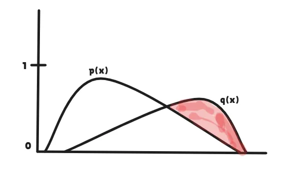
Now that you’re seeing this, you may perceive why we aren’t sampling instantly from the q(x) likelihood distribution, proper? However truthfully, there isn’t any data loss right here. This course of permits us to pattern solely from the portion the place correction is required. Therefore, for this reason speculative decoding is taken into account mathematically lossless.
So, now we formally perceive how speculative decoding truly works. Woohoo. Now, let’s dive into the final part of this weblog.
Totally different Approaches to Speculative Decoding
Strategy 1
On this strategy, we observe the identical technique that we carried out within the earlier examples, i.e., utilizing two completely different fashions. These fashions can belong to the identical organisation (like Meta, Mistral, and many others.) or may also be from completely different organisations. The draft mannequin generates Okay tokens directly, and the goal mannequin verifies all these tokens in a single ahead move. When all of the draft tokens are accepted, we successfully advance Okay tokens for the price of one massive ahead move.
Eg, we are able to use 2 fashions from the identical organisation:
- mistralai/Mistral-7B-v0.1 → mistralai/Mixtral-8x7B-v0.1
- deepseek-ai/deepseek-llm-7b-base → deepseek-ai/deepseek-llm-67b-base
- Qwen/Qwen-7B → Qwen/Qwen-72B
We are able to additionally use fashions from completely different organisations:
- meta-llama/Llama-2-7b-hf → Qwen/Qwen-72B
- meta-llama/Llama-2-13b-hf → Qwen/Qwen-72B-Chat
NOTE: Simply remember the fact that cross-organisation setups normally have decrease token acceptance charges attributable to tokeniser and distribution mismatch, so the speedups could also be smaller in comparison with same-family pairs. It’s usually most well-liked to make use of fashions from the identical household.
Strategy 2
For some use circumstances, internet hosting two separate fashions might be memory-intensive. In such situations, we are able to undertake the technique of self-speculation, the place the identical mannequin is used for each drafting and verification.
This doesn’t imply we actually use two separate situations of the identical mannequin. As a substitute, we modify the mannequin to behave like a smaller model through the draft part. This may be achieved by lowering precision (e.g., lower-bit representations) or by selectively utilizing solely a subset of layers.
1. LayerSkip (Early Exit)
On this strategy, we use solely a subset of the mannequin’s layers (e.g., Layer 1 to 12) repeatedly as a light-weight draft mannequin for Okay instances, and infrequently run the complete mannequin (e.g., Layer 1 to 32) as soon as to confirm all of the drafted tokens. In apply, the partial mannequin is run Okay instances to generate Okay draft tokens, after which the complete mannequin is run as soon as to confirm them. This acts as a less expensive drafting mechanism whereas nonetheless sustaining output high quality throughout verification. This strategy usually achieves round 2x to 2.5x speedup with an acceptance charge of 75-80%.
2. EAGLE
EAGLE (Extrapolation Algorithm for Better Language-Mannequin Effectivity) is a realized predictor strategy, the place a small auxiliary mannequin (approx 100M parameters) is educated to foretell draft tokens primarily based on the frozen mannequin’s hidden states. This achieves round 2.5x to 3x speedup with an acceptance charge of 80-85%.
EAGLE basically acts like a pupil mannequin used for drafting. It removes the overhead of operating a totally separate massive draft mannequin, whereas nonetheless permitting the goal mannequin to confirm a number of tokens in parallel.
One other plus level of utilizing self-speculation is that there isn’t any latency overhead since we don’t change fashions right here. We are able to discover EAGLE and different speculative decoding methods in additional element in a separate weblog.
Conclusion
Speculative decoding works finest with low batch sizes, underutilised GPUs, and lengthy outputs (100+ tokens). It’s particularly helpful for predictable duties like code technology and latency-sensitive functions the place sooner responses matter.
It hurries up inference by drafting tokens and verifying them in parallel, lowering latency with out dropping high quality. Rejection sampling retains outputs an identical to the goal mannequin. New approaches like LayerSkip and EAGLE additional enhance effectivity, making this a sensible technique for scaling LLM efficiency.
Continuously Requested Questions
A. It’s a technique the place a smaller mannequin drafts tokens and a bigger mannequin verifies them to hurry up textual content technology.
A. It generates a number of tokens directly and verifies them in parallel as an alternative of processing one token per ahead move.
A. Tokens are accepted if q(x) ≥ p(x), in any other case accepted probabilistically utilizing min(1, q(x)/p(x)).
I specialise in reviewing and refining AI-driven analysis, technical documentation, and content material associated to rising AI applied sciences. My expertise spans AI mannequin coaching, knowledge evaluation, and knowledge retrieval, permitting me to craft content material that’s each technically correct and accessible.
Login to proceed studying and revel in expert-curated content material.